Problems 1. The Orange Octagon Discount Department Store sells snowblowers during
the winter months. Snowblowers cost $175.00 each and sell for $395.00. The
manager knows that the volume of sales is not large, as indicated by the
following data on the number of snowblowers that were sold in each week
during the past two selling seasons, which contained 20 weeks each: 0, 1,
3, 1, 2, 0, 3, 4, 2, 1, 4, 2, 0, 2, 0, 0, 2, 0, 1. 3, 1, 1, 1, 3, 3, 2,
2, 0, 4, 1, l, 0, 2, 2, 0, 1, 3, 1, 3 snowblowers. The manager has decided
to start the season with four snowblowers on hand. Only snowblowers on hand
at the beginning of the week can be sold. Additional snowblowers can be
ordered from the supplier, with a two-week lead time, and the manager plans
to order two of them whenever the quantity on hand falls to two or less
at the end of the week. Use the random numbers that follow to simulate this
policy for 10 weeks: 491, 631, 139, 502, 006, 856, 904, 91, 821, 757. - What is the empirical probability distribution for the weekly sales
of snowblowers?
- What random numbers go with each value of the random variable?
- Construct a table in the style of Example 19S-2b(2) in your textbook,
showing the history of the inventory of snowblowers for
the 10-week period.
- How many snowblowers were sold? How much gross margin was made?
- How many sales were lost? What was the dollar amount of the loss?
- What is your evaluation of the policy?
2. The number of ambulance calls can be represented by a Poisson distribution
with a mean of four per day. Obtain the Poisson distribution from Table
C in the Appendix and use the following random numbers to simulate six days
of ambulance calls: 005, 820, 471, 187, 177, 341. - a. Which random numbers go with each value of the random variable?
- Construct a table in the style of Solved Problem I in your textbook to
show the history of the six days.
3. The daily sales of unleaded gasoline at the self-serve pump can be represented
by a normal curve with a mean of 300 gallons and a standard deviation of 30
gallons. Use row 8, columns 1, 2, 3, 4, in Table 19S-2 in your textbook to simulate
four days of gasoline sales. 4. (One step beyond) Use an EXCEL spreadsheet to simulate ten days of gasoline
sales for the self-serve pump in problem #3. This will require the use of EXCEL's
Analysis ToolPak VBA. To see if it is installed in your system, click on TOOLS
and look for Data Analysis at the bottom of the list. If it is there, you are
ready to proceed. If not, click on Add-Ins and select Analysis ToolPak VBA.
Data Analysis should now appear in your TOOLS menu. - How should the problem be entered on the spreadsheet?
- What are the daily sales?
5. The length of time which a customer spends pumping gasoline at the self-serve
pump can be represented by a negative exponential distribution with a mean of
2 minutes. Use these four random numbers to simulate four customers pumping
gasoline: 84275, 07523, 33362, 64270. - What is the value of
 <a onClick="window.open('/olcweb/cgi/pluginpop.cgi?it=gif::Image398::/sites/dl/free/0072443901/24520/Image398.gif','popWin', 'width=NaN,height=NaN,resizable,scrollbars');" href="#"><img valign="absmiddle" height="16" width="16" border="0" src="/olcweb/styles/shared/linkicons/image.gif">Image398 (0.0K)</a>Image398 ? <a onClick="window.open('/olcweb/cgi/pluginpop.cgi?it=gif::Image398::/sites/dl/free/0072443901/24520/Image398.gif','popWin', 'width=NaN,height=NaN,resizable,scrollbars');" href="#"><img valign="absmiddle" height="16" width="16" border="0" src="/olcweb/styles/shared/linkicons/image.gif">Image398 (0.0K)</a>Image398 ? - What are the four times?
6. (One step beyond) The plant manager believes that in the production of fluorescent
light tubes, 6 percent will turn out to be defective; the remainder will be satisfactory.
Use rows 10-12 in Table 19S-1 in your textbook to simulate the production of 36
fluorescent light tubes.
- Which random numbers go with each type of fluorescent tube?
- What is the sequence of satisfactory (S) and defective (D) tubes.
- What percent of the 36 tubes are defective?
- Is the plant manager mistaken in the 6% figure?
1. a, b. | x | f | p | Cumulative Probability | Random Numbers | | | 0 1 2 3 4 | 9 12 9 7 3 | .225 .300 .225 .175 .075 | .225 .525 .750 .925 1.000 | 001-225 226-525 526 750 751-925 926-000 | | | Totals | 40 | 1.000 | | |
c. | Week | Random Number | Demand | Sales | Quantity Ordered | Quantity Received | | | 1 2 3 4 5 6 7 8 9 10 | 491 631 139 502 006 856 904 091 821 757 | 1* 2 0 1 0 3 3 0 3 3 | 1 2 0 1 0 3 3 0 0*** 2 | 0 2 2** 2 0 0 2 2 0 2 | 0 0 0 2 2 2 0 0 2 2 | | | Totals | | 16 | 12 | | |
*491 comes between 226 and 525 and designates X = 1. **Since the inventory contains 1 snowblower at the end of the third week. ***Because the beginning inventory is 0. | | Week | Beginning Inventory | Sales | Receipts | Ending Inventory | | | 1 2 3 4 5 6 7 8 9 10 | 4 3 1 1 2 4 3 0 0 2 | 1 2 0 1 0 3 3 0 0 2 | 0 0 0 2 2 2 0 0 2 2 | 3 1 1 2 4 3 0 0 2 2 |
d. The total of the sales column is 12 snowblowers. The gross margin = 12(395
- 175) = $2,640.e. The difference between the total of the demand column and
the total of the sales column is 4 snowblowers. The gross margin lost = 4(395
- 175) = $880.
f. While 10 weeks is a very small sample, a tentative hypothesis is that more
snowblowers could be sold if the order quantity were increased. 2. a. | | Number | Cumulative | Random | | | of Calls | Probability | Number Range | | | 0 | .018 | 001 018 | | | 1 | .092 | 019 - 092 | | | 2 | .238 | 093 - 238 | | | 3 | .433 | 239 - 433 | | | 4 | .629 | 434 - 629 | | | 5 | .785 | 630 - 785 | | | 6 | .889 | 786 - 889 | | | 7 | .949 | 890 - 949 | | | 8 | .979 | 950 - 979 | | | 9 | .992 | 980 - 992 | | | 10 | .997 | 993 - 997 | | | 11 | .999 | 998 - 999 | | | 12 | 1.000 | 1,000 |
b. | | Random | Number | | | Day | Number | of Calls | | | 1 | 005 | 0* | | | 2 | 820 | 6 | | | 3 | 471 | 4 | | | 4 | 187 | 2 | | | 5 | 177 | 2 | | | 6 | 341 | 3 |
*005 comes between 001 and 018 and designates X = 0. 3. | Day | Random Number | Sales | | | 1 2 3 4 | 2.40 0.38 - 0.15 - 1.04 | 372.00* 311.40 295.50 268.80 |
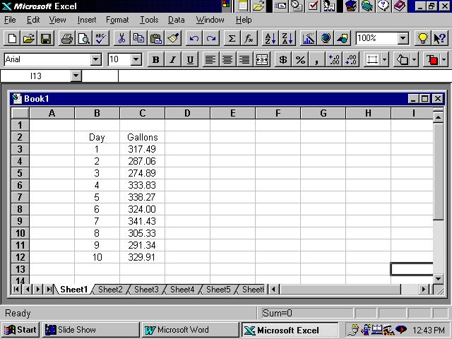
*Sales = Mean + (R.N.)(standard deviation) = 300 + (2.40)(30) = 372.00 gal. - a. Click on TOOLS; DATA ANALYSIS; RANDOM NUMBER GENERATOR. Number of Variables
= 1; Number of Random Numbers = 10; Distribution = Normal; Mean = 300; Standard
Deviation = 30; Random Seed = 1776*; Output Range = C3:C12.
b.  <a onClick="window.open('/olcweb/cgi/pluginpop.cgi?it=gif::Image399::/sites/dl/free/0072443901/24520/Image399.gif','popWin', 'width=NaN,height=NaN,resizable,scrollbars');" href="#"><img valign="absmiddle" height="16" width="16" border="0" src="/olcweb/styles/shared/linkicons/image.gif">Image399 (21.0K)</a>Image399 . <a onClick="window.open('/olcweb/cgi/pluginpop.cgi?it=gif::Image399::/sites/dl/free/0072443901/24520/Image399.gif','popWin', 'width=NaN,height=NaN,resizable,scrollbars');" href="#"><img valign="absmiddle" height="16" width="16" border="0" src="/olcweb/styles/shared/linkicons/image.gif">Image399 (21.0K)</a>Image399 .
*NOTE: The choice of a value for the Seed Number is arbitrary. Experiment
with some other seeds, such as your birthday in the form of 62180, perhaps.
5. a. The service time: 1/l = 2 minutes, and l = .50. b. p(T) = exp(- 0.5t), and t = - (1/l)(ln(.RN)). c. | Week | Random Number | ln(.RN) | Pumping Time (min.)* | | | 1 2 3 4 | .84275 .07523 .33362 .64270 | - 0.1711 - 2.5872 - 1.0978 - 0.4421 | 0.3422 5.1744 2.1958 0.8842 |
*Pumping Time = - 2×ln(.RN) 6. a. | Type of Tube | Random Number Range | | | Satisfactory Defective | 01-94 95-100 |
b. Reading Table 19S-1 horizontally: S S S S S S S S S S S S S S S S S S S
S S S S D S S S S S S S S S S S S.
c. p = 1/36 = 2.78%.
d. Not necessarily; the 6% defective tubes will occur over the long run but
not for any very short period. (For the statistician: the standard error of
the sample percent, if the true percent of defective tubes is, in fact, 6% is
3.96% and it is easy to draw a sample with p = 2.78% from a population with
6% defective items.) |


