Student Center | Instructor Center | Information Center | Home

Statistics for the Behavioral Sciences, 4/e

Michael Thorne, Mississippi State University -- Mississippi State
Martin Giesen, Mississippi State University -- Mississippi State

Graphing Data

SPSS Exercises

USING SPSS-EXAMPLE AND EXERCISES
If you haven't already done so, read Appendix 4 before proceeding with these exercises.

SPSS has a variety of graphing capabilities, both within certain procedures and independently under the Graphs menu. Unfortunately, the available choices for graphs may not correspond exactly to the ones requested in this chapter and described in the textbook. Thus, you may have to choose a graph that is an approximation to the one requested or one that may require you to draw a few lines to achieve the desired result.

Example: We will use SPSS to produce graphs for Problem 1. In this problem, part a requests a frequency polygon, and a histogram is requested in part b. SPSS won't easily produce either of these graphs exactly as we have defined them in the text. However, a good approximation for the frequency polygon is provided by an SPSS line graph constructed as follows:

Start SPSS, enter the data, and name the variable test. Again, remember that when we enter data from a frequency distribution, each score must be entered the number of times indicated by its frequency.
Click Graphs>Line>Simple>Summaries for groups of cases>Define.
Highlight and move the variable test into the Category Axis box and be sure "N of cases" is indicated in the Line Represents box. The Define Simple Line dialog box should appear as follows:
Click OK and the graph should appear in the output Viewer window.
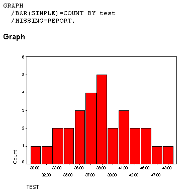
To approximate a histogram for part b, click Graphs>Bar>Simple>Summaries for groups of cases> Define.
Move test into the Category Axis box and be sure "N of cases" is indicated. The dialog box should appear as shown in step 3 except that the box is labeled as Define Simple Bar rather than Define Simple Line.
Click OK and the graph appears in the output Viewer window.
To construct a cumulative frequency curve for part c, repeat steps 2-4 except choose "Cum. N of cases" rather than "N of cases" in the Line Represents box.
To construct a cumulative percentage curve for part d, repeat steps 2-4 except choose "Cum. % of cases."

Note that SPSS does not graph values with 0 frequency. For example, in the first graph in which we used an SPSS line graph to approximate the frequency polygon, you can see that the horizontal axis does not show the score of 31 and the line does not drop back to the X axis to indicate a frequency of 0 for that score. The same is true of the other graphs, and this is one way that SPSS approximates the graphs as we defined them in the text.

The output showing the four graphs for Problem 1 should appear as follows. (Again, note that SPSS does not usually plot scores with a frequency of zero.)

Exercises Using SPSS

Create a line graph using the data in Problem 2. Because of the way the data are provided, we have some special instructions for you to use to "trick" SPSS into giving the graph we want you to produce. Enter the data as a separate variable for day and as another separate variable for the frequency that you should call freqcig. The steps are as follows:
1. Click Graphs>Line>Simple>Values of individual cases>Define.
2. In the Define Simple Line dialog box, freqcig should be in the Line Represents box and day should be in the Category Labels Variable box.
3. Click OK and the graph should appear in the output Viewer window.
Create a stem-and-leaf plot of the speeds of cars given in Problem 8. Again, we need to provide some special instructions for where to look for the stem-and-leaf plot in SPSS. The instructions are as follows:
1. Start SPSS, enter the data, and name the variable speeds.
2. The stem-and-leaf plot is a plot option under the Explore procedure. Click as follows:
  Analyze>Descriptive Statistics>Explore.
  In the Explore dialog box, move speeds to the Dependent List and click Plots in the Display box (lower left).
  Click Plots (lower right) to open the Explore: Plots dialog box. Be sure "stem-and-leaf" is checked and None is checked under Boxplots (it won't hurt if you leave it), then click Continue.
  In the Explore dialog box, click OK and the output should appear.

Click here to view the answers. (35.0K)

2003 McGraw-Hill Higher Education
Any use is subject to the Terms of Use and Privacy Notice.
McGraw-Hill Higher Education is one of the many fine businesses of The McGraw-Hill Companies.